A Guide to Approximations, By Jack Ganssle
Need fast C code for computing trig functions (sin, cos, tan, atan, acos and asin)? That included with the runtime library might not be fast enough. This article gives C code for these functions optimized for speed.
This is available in Spanish here. And there's another article about approximations for other functions like roots, exponentials and logs here.
Most embedded processors don't know how to compute trig and other complex functions. Programming in C we're content to call a library routine that does all of the work for us. Unhappily this optimistic approach often fails in real time systems where size, speed and accuracy are all important issues.
The compiler's runtime package is a one-size-fits-all proposition. It gives a reasonable trade-off of speed and precision. But every embedded system is different, with different requirements. In some cases it makes sense to write our own approximation routines. Why?
Speed - Many compilers have very slow runtime packages. A clever approximation may eliminate the need to use a faster CPU.
Predictability - Compiler functions vary greatly in execution time depending on the input argument. Real time systems must be predictable in the time domain. The alternative is to always assume worst case execution time, which again may mean your CPU is too slow, too loaded, for the application.
Accuracy - Read the compiler's manuals carefully! Some explicitly do not support the ASNI C standard, which requires all trig to be double precision. (8051 compilers are notorious for this). Alternatively, why pay the cost (in time) for double precision math when you only need 5 digits of accuracy?
Size - When memory is scarce, using one of these approximations may save much code space. If you only need a simple cosine, why include the entire floating point trig library?
This collection is not an encyclopedia of all possible approximations; rather, it's the most practical ones distilled from the bible of the subject, Computer Approximations by John Hart (ISBN 0-88275-642-7). Unfortunately this work is now out of print. It's also very difficult to use without a rigorous mathematical background.
All of the approximations here are polynomials, or ratios of polynomials. All use very cryptic coefficients derived from Chebyshev series and Bessel functions. Rest assured that these numbers give minimum errors for the indicated ranges. Each approximation (with a few exceptions) has an error chart so you can see exactly where the errors occur. In some cases, if you're using a limited range of input data, your accuracies can far exceed the indicated values. For instance, cos_73 is accurate to 7.3 decimal digits over the 0 to 360 degree range. But as the graph shows, in the range 0 to 30 degrees you can get almost an order of magnitude improvement.
Do be wary of the precision of your compiler's floating point package. Some treat doubles as floats. Others, especially for tiny CPUs like the PIC, cheat and offer less than full 32 bit floating point precision.
All of the code for the following approximations was compiled with Microsoft's Visual C++ 6.0. The source is available at www.ganssle.com/approx/sincos.cpp. It includes test code that writes a text file of results and errors; imported to a spreadsheet we can see just how accurate they are. The code in this article is extracted from that file.
General Trig Notes
We generally work in radians rather than degrees. The 360 degrees in a circle are equivalent to 2Π radians; thus, one radian is 360/(2Π), or about 57.3 degrees. This may seem a bit odd till you think of the circle's circumference, which is 2Πr; if r (the circle's radius) is one, the circumference is indeed 2 Π.
The conversions between radians and degrees are:
Angle in radians= angle in degrees * 2 Π /360
Angle in degrees= angle in radians * 360/(2 Π)
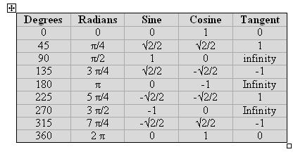
Cosine and Sine
The following examples all approximate the cosine function; sine is derived from cosine via the relationship:
sin(x)=cos(Π/2-x)
In other words, the sine and cosine are the same function, merely shifted 90° in phase. The sine code is (assuming we're calling cos_32, the lowest accuracy cosine approximation):

All of the cosine approximations in this chapter compute the cosine accurately over the range of 0 to Π/2 (0 to 90°). That surely denies us of most of the circle! Approximations in general work best over rather limited ranges; it's up to us to reduce the input range to something the approximation can handle accurately.
Therefore, before calling any of the following cosine approximations we assume the range has been reduced to 0 to Π/2 using the following code:
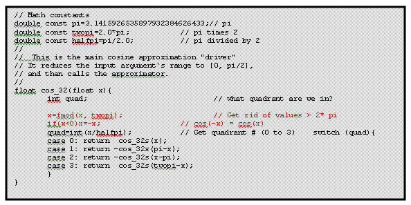
This code is configured to call cos_32s, which is the approximation (detailed shortly) for computing the cosine to 3.2 digits accuracy. Use this same code, though, for all cosine approximations; change cos_32s to cos_52s, cos_73s or cos_121s, depending on which level of accuracy you need. See the complete listing for a comprehensive example.
If you can guarantee that the input argument will be greater than zero and less than 2 Π, delete the two red lines in the listing above to get even faster execution.
Be clever about declaring variables and constants. Clearly, working with the cos_32 approximation nothing must be declared "double". Use float for more efficient code. Reading the complete listing you'll notice that for cos_32 and cos_52 we used floats everywhere; the more accurate approximations declare things as doubles.
One trick that will speed up the approximations is to compute x2 by incrementing the characteristic of the floating point representation of x. You'll have to know exactly how the numbers are stored, but can save hundreds of microseconds over performing the much clearer "x*x" operation.
How does the range reduction work? Note that the code divides the input argument into one of four "quadrants" - the very same quadrants of the circle shown below:
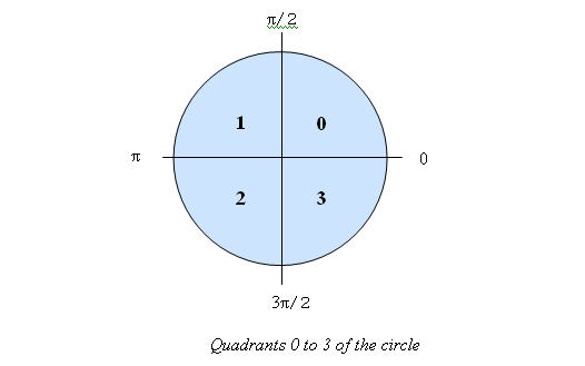
- For the first quadrant (0 to Π/2) there's nothing to do since the cosine approximations are valid over this range.
- In quadrant 1 the cosine is symertrical with quadrant 0, if we reduce it's range by subtracting the argument from Π. The cosine, though, is negative for quadrants 1 and 2 so we compute -cos(Π-x).
- Quadrant 2 is similar to 1.
- Finally, in 3 the cosine goes positive again; if we subtract the argument from 2 Π it translates back to something between 0 and Π/2.
The approximations do convert the basic polynomial to a simpler, much less computationally expensive form, as described in the comments. All floating point operations take appreciable amounts of time, so it's important to optimize the design.
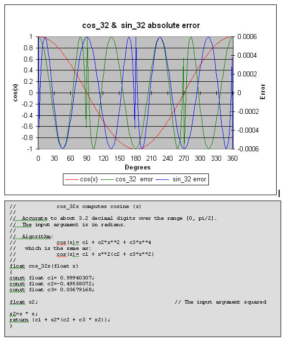
cos_32 computes a cosine to about 3.2 decimal digits of accuracy. Use the range reduction code (listed earlier) if the range exceeds 0 to Π/2. The plotted errors are absolute (not percent error).
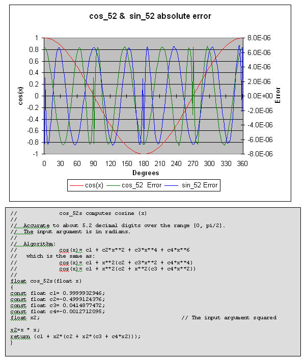
cos_52 computes a cosine to about 5.2 decimal digits of accuracy. Use the range reduction code (listed earlier) if the range exceeds 0 to Π/2. The plotted errors are absolute (not percent error).
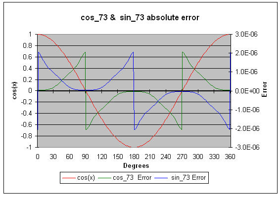
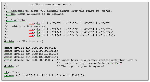
cos_73 computes a cosine to about 7.3 decimal digits of accuracy. Use the range reduction code (listed earlier) if the range exceeds 0 to Π/2. Also plan on using double precision math for the range reduction code to avoid losing accuracy. The plotted errors are absolute (not percent error).
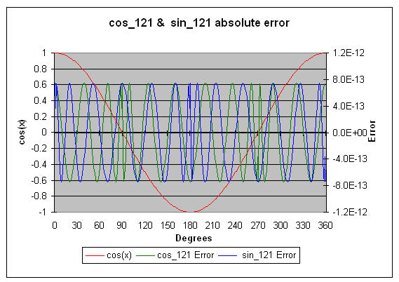
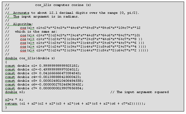
cos_121 computes a cosine to about 12.1 decimal digits of accuracy. Use the range reduction code (listed earlier) if the range exceeds 0 to Π/2. Also plan on using double precision math for the range reduction code to avoid losing accuracy. The plotted errors are absolute (not percent error).
Higher Precision Cosines
Given a large enough polynomial there's no limit to the possible accuracy. A few more algorithms are listed here. These are all valid for the range of 0 to Π/2, and all can use the previous range reduction algorithm to change any angle into one within this range. All take an input argument in radians.
No graphs are included because these exceed the accuracy of the typical compiler's built-in cosine function. . . . so there's nothing to plot the data against.
Note that C's double type on most computers carries about 15 digits of precision. So for these algorithms, especially for the 20.2 and 23.1 digit versions, you'll need to use a data type that offers more bits. Some C's support a long double. But check the manual carefully! Microsoft's Visual C++, for instance, while it does support the long double keyword, converts all of these to double.
Accurate to about 14.7 decimal digits over the range [0, Π/2]:
               c1= 0.99999999999999806767
               c2=-0.4999999999998996568
               c3= 0.04166666666581174292
               c4=-0.001388888886113613522
               c5= 0.000024801582876042427
               c6=-0.0000002755693576863181
               c7= 0.0000000020858327958707
               c8=-0.000000000011080716368
               cos(x)= c1 + x2(c2 + x2(c3 + x2(c4 + x2(c5 +
                            x2(c6 + x2(c7 + x2*c8))))))
Accurate to about 20.2 decimal digits over the range [0, Π/2]:
      c1 = 0.9999999999999999999936329
      c2 =-0.49999999999999999948362843
      c3 = 0.04166666666666665975670054
      c4 =-0.00138888888888885302082298


      c6 =-0.00000027557319209666748555
      c7 = 0.0000000020876755667423458605
      c8 =-0.0000000000114706701991777771
      c9 = 0.0000000000000477687298095717
      c10=-0.00000000000000015119893746887
  cos(x)= c1 + x2(c2 + x2(c3 + x2(c4 + x2(c5 + x2(c6 +
               x2(c7 + x2(c8 + x2(c9 + x2*c10))))))))
Accurate to about 23.1 decimal digits over the range [0, Π/2]:
       c1 = 0.9999999999999999999999914771
       c2 =-0.4999999999999999999991637437
       c3 = 0.04166666666666666665319411988
       c4 =-0.00138888888888888880310186415
       c5 = 0.00002480158730158702330045157
       c6 =-0.000000275573192239332256421489
       c7 = 0.000000002087675698165412591559
       c8 =-0.0000000000114707451267755432394
       c9 = 0.0000000000000477945439406649917
       c10=-0.00000000000000015612263428827781
       c11= 0.00000000000000000039912654507924
   cos(x)= c1 + x2(c2 + x2(c3 + x2(c4 + x2(c5 + x2(c6 +
                x2(c7 + x2(c8 + x2(c9 + x2(c10 + x2*c11)))))))))
Tangent
The tangent of an angle is defined as tan(x)=sin(x)/cos(x). Unhappily this is not the best choice, though, for doing an approximation. As cos(x) approaches zero the errors propagate rapidly. Further, at some points like Π/4 (see the previous graphs of sine and cosine errors) the errors of sine and cosine reinforce each other; both are large and have the same sign.
So we're best off using a separate approximation for the tangent. All of the approximations we'll use generate a valid tangent for angles in the range of 0 to Π/4 (0 to 45 degrees), so once again a range reduction function will translate angles to this set of values.
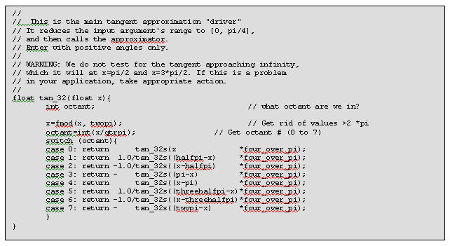
The code above does the range reduction and then calls tan_32. When using the higher precision approximations substitute the appropriate function name for tan_32.
The reduction works much like that for cosine, except that it divides the circle into octants and proceeds from there. One quirk is that the argument is multiplied by 4/Π. This is because the approximations themselves actually solve for tan((Π/4)x).
The listings that follow give the algorithms needed.
Remember that tan(90) and tan(270) both equal infinity. As the input argument gets close to 90 or 270 the value of the tangent skyrockets, as illustrated on the following error charts. Never take a tangent close to 90 or 270 degrees!
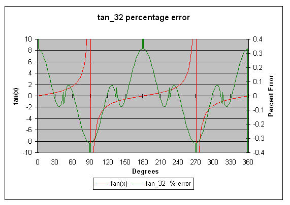
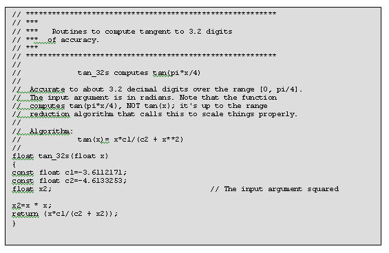
tan_32 computes the tangent of Π/4*x to about 3.2 digits of accuracy. Use the range reduction code to translate the argument to 0 to Π/4, and of course to compensate for the peculiar "Π/4" bias required by this routine. Note that the graphed errors are percentage error, not absolute.
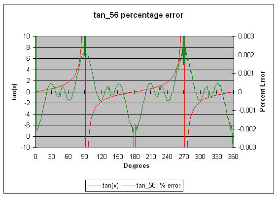
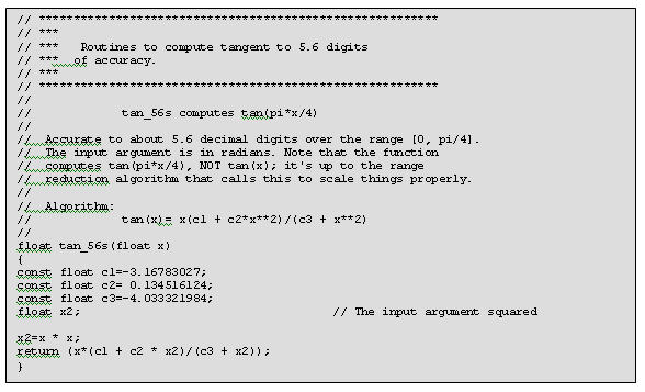
tan_56 computes the tangent of Π/4*x to about 5.6 digits of accuracy. Use the range reduction code to translate the argument to 0 to Π/4, and of course to compensate for the peculiar "Π/4" bias required by this routine. Note that the graphed errors are percentage error, not absolute.
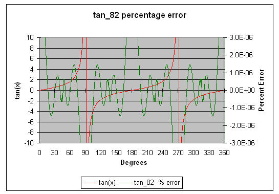
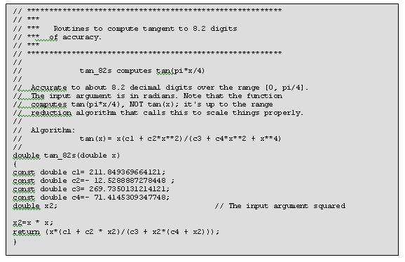
tan_82 computes the tangent of Π/4*x to about 8.2 digits of accuracy. Use the range reduction code to translate the argument to 0 to Π/4, and of course to compensate for the peculiar "Π/4" bias required by this routine. Note that variables are declared as "double". The graphed errors are percentage error, not absolute.
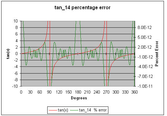
tan_141 computes the tangent of Π/4*x to about 14.1 digits of accuracy. Use the range reduction code to translate the argument to 0 to Π/4, and of course to compensate for the peculiar "Π/4" bias required by this routine. Note that variables are declared as "double". The graphed errors are percentage error, not absolute.
Higher Precision Tangents
Given a large enough polynomial there's no limit to the possible accuracy. A few more algorithms are listed here. These are all valid for the range of 0 to Π/4, and all should use the previous range reduction algorithm to change any angle into one within this range. All take an input argument in radians, though it is expected to be mangled by the Π/4 factor. The prior range reducer will correct for this.
No graphs are included because these exceed the accuracy of the typical compiler's built-in cosine function . . .. so there's nothing to plot the data against.
Note that C's double type on most computers carries about 15 digits of precision. So for these algorithms, especially for the 20.2 and 23.1 digit versions, you'll need to use a data type that offers more bits. Some C's support a long double. But check the manual carefully! Microsoft's Visual C++, for instance, while it does support the long double keyword, converts all of these to double.
Accurate to about 20.3 digits over the range of 0 to Π/4:
    c1= 10881241.46289544215469695742
    c2=-  895306.0870564145957447087575
    c3=    14181.99563014366386894487566
    c4=-      45.63638305432707847378129653
    c5= 13854426.92637036839270054048
    c6=- 3988641.468163077300701338784
    c7=   135299.4744550023680867559195
    c8=-    1014.19757617656429288596025
  tan(xΠ/4)=x(c1 + x2(c2 + x2(c3 + x2*c4)))
            /(c5 + x2(c6 + x2(c7 + x2(c8 + X2))))
Accurate to about 23.6 digits over the range of 0 to Π/4: c1= 4130240.588996024013440146267 c2=- 349781.8562517381616631012487 c3= 6170.317758142494245331944348 c4=- 27.94920941380194872760036319 c5= 0.0175143807040383602666563058 c6= 5258785.647179987798541780825 c7=-1526650.549072940686776259893 c8= 54962.51616062905361152230566 c9=- 497.495460280917265024506937 tan(xΠ/4)=x(c1 + x2(c2 + x2(c3 + x2(c4 + x2*c5)))) /(c6 + x2(c7 + x2(c8 + x2(c9 + x2))))
Arctangent, arcsine and arccosine
The arctangent is the same as the inverse tangent, so arctan(tan(x))=x. It's often denoted as "atan(x)" or "tan-1(x)".
In practice the approximations for inverse sine an cosine aren't too useful; mostly we derive these from the arctangent as follows:
Arcsine(x)	= atan(x/√(1-x2))
Arccosine(x)	= Π/2 - arcsine(x)
             = Π/2 - atan(x/√(1-x2))
The approximations are valid for the range of 0 to Π /12. The following code, based on that by Jack Crenshaw in his Math Toolkit for Real-Time Programming, reduces the range appropriately:
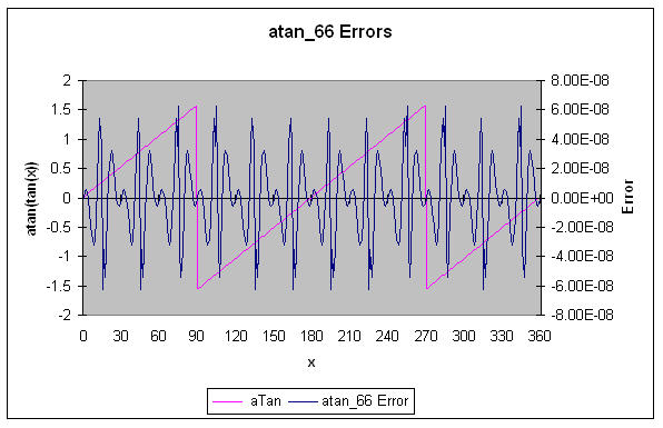
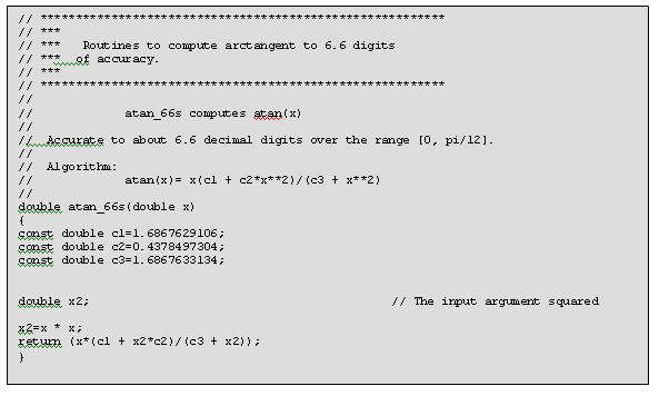
atan_66 computes the arctangent to about 6.6 decimal digits of accuracy using a simple rational polynomial. It's input range is 0 to Π /12; use the previous range reduction code.
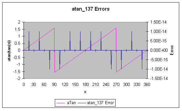
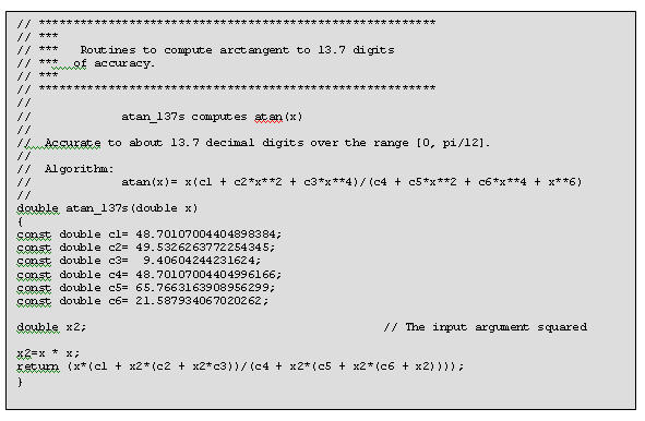
atan_137 computes the arctangent to about 13.7 decimal digits of accuracy using a simple rational polynomial. It's input range is 0 to Π /12; use the previous range reduction code.
(Please use proper engineering analysis when implementing these suggestions - no guarantees are given).

