By Jack Ganssle

Fourier And Us

Published December 2013 on embedded.com

In my seminars I often talk about the importance of understanding at least a little electromagnetics theory, even for purely firmware people. But the subject is hard to understand and sometimes harder to believe, which is why the best book on the subject, "High Speed Digital Design," is subtitled "A Handbook of Black Magic."

Why is it important? You'll surely be probing your design with various tools like scopes and logic analyzers, and every such probe has some impedance. As speeds get higher, that impedance is ever more likely to corrupt the operation of the device.

But "speed" is poorly understood today. We equate clock rate with speed, which is only part of the story.

Almost two hundred years ago polymath Jean-Baptiste Joseph Fourier showed that any periodic function can be expressed as the sum of sine waves of different amplitudes and frequencies. A square wave, like a microprocessor clock, is periodic and its Fourier series is:

In other words, a square wave is composed of the sum of the sine of the wave's frequency and each of its odd harmonics. (A harmonic is an integer multiple of the base frequency.) As you can see, no matter what the square wave's frequency is, it has harmonics that go to infinity, though at progressively lower amplitudes.

A useful rule of thumb is that for most digital design we can ignore harmonics that exceed:

Where Tr is the square wave's rise time in nanoseconds. Every real-world signal takes time to transition from a zero to a one. Above f the Fourier components are down about 40 dB.

Since a picture is worth a million bits, look at the following scope trace:

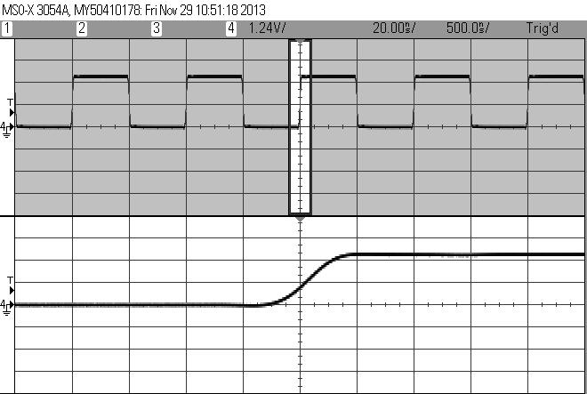
A square wave with 20 ns rise time.

The top trace is a 1 MHz square wave, just like a CPU clock. The bottom is an expanded view of the highlighted portion of the same trace. Note that what looks like a nice, quick zero to one transition actually takes quite a bit of time. In this case the rise time is 20 ns. Running 20 ns through the previous formula and it's clear that anything above 25 MHz will be so far down we don't have to worry about them. But it does mean that 1 MHz signal has important frequency components that far exceed the fundamental.

That square wave comes from my scope's waveform generator. To show the Fourier effect more dramatically I built a circuit to improve the signal's rise time by feeding the signal through a fast gate.

It is possible to see the individual frequency components predicted by the Fourier series. Most modern scopes can compute the Fourier transform of a signal, as in the following screen capture.

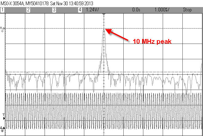
10 MHz sine wave

The bottom trace is a simple 10 MHz sine wave. Above it is the Fourier transform. Unlike a normal scope display where the horizontal axis is time and the vertical volts, the upper one is displayed in units of dB and frequency. In this case the screen's scale is set to 0 MHz at the left and 20 MHz all the way to the right. Note there's a very strong peak exactly at 10 MHz, because 10 MHz is the only frequency component in a 10 MHz sine wave. Sure, there are some other things running around on that trace due to an imperfect waveform generator and some artifacts of the Fourier transform process. But the ugly stuff is 57 dB lower than the peak. That's 1/500,000 less than the 10 MHz peak. Switching from dB to voltage makes this more obvious:

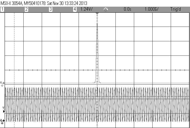
10 MHz sine wave in volts.

Here's the Fourier transform of the 20 ns rise time square wave:

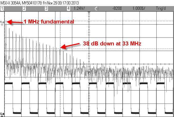
Spectrum of a square wave with 20 ns rise time.

The bottom trace is the 1 MHz square wave from the scope's waveform generator, before going to the fixer-upper circuit. Above it is the Fourier transform. In this case the screen's scale is set to 0 MHz at the left and 100 MHz at the right. Each peak is one of the square wave's odd harmonics from the Fourier series.

Unsurprisingly, the highest peak is at the wave's fundamental frequency of 1 MHz. At 33 MHz the signal is down 38 dB, and quickly rolls off from there. That's close enough to the rule of thumb for practical work.

With the fixer-upper circuit the rise time is now 1 ns:

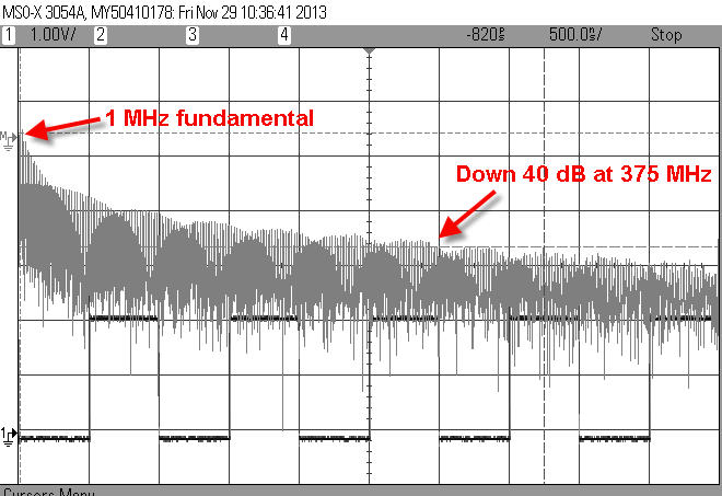
Spectrum of a square wave with 1 ns rise time.

This looks different from the previous picture because now the Fourier transform window goes from 0 MHz to 500 MHz. There are a lot more harmonics displayed. But notice that the 40 dB point is now at 375 MHz (the formula predicts 500 MHz, again, close enough for a rule of thumb). It's important to remember that this is the spectrum of the same 1 MHz signal; all that has changed is the rise time.

If your little 8 bit system is clocking at just a few MHz, or even hundreds of KHz, with sharp edges it may have all of the same high speed issues we usually attribute to much faster circuits.

Sounds hard to believe. Some time ago a company asked for help with their 30 year old, 4 MHz, Z80 design. A new batch of boards didn't work, though the design was unchanged. It seems the semiconductor vendor had increased the speed of some of the logic. Those gates that used to switch in 15 ns now did it in 5. The company had to redesign this board as a high-speed digital system simply because of the faster rise time.

The takeaway is that we can't think of digital signals as we do simple sine waves. They are composed of a lot of harmonics, and, depending on rise time, those harmonics can have a huge effect on the circuit's operation. A 1 MHz clock does not necessarily imply a slow circuit.

Free Embedded Muse newsletter - twice/monthly, hard-hitting technical info that goes to 48,000+ engineers. Click here to sign up or enter your email here: