Electromagnetics for Firmware People

Maxwell's Laws really are important for firmware development. Here is an introduction.

Published in Embedded Systems Programming

For hints, tricks and ideas about better ways to build embedded systems, subscribe to The Embedded Muse, a free biweekly e-newsletter. No hype, just down to earth embedded talk. 23,000 other engineers subscribe. It takes just a few seconds (all we need is your email address, which is shared with absolutely no one) to subscribe to the Embedded Muse.

Electromagnetics for Firmware People

Programming classes and circuit theory were a breeze for me as an EE student at the University of Maryland many years ago. Math was a bit more of a struggle, especially the more advanced classes like abstract algebra. But the two required electromagnetics classes were killers.

I had no idea what the professors were babbling about. Orthogonal E and B fields sounded pretty simple until instantiated into the baffling form of Maxwell's Laws.

Maxwell said a lot of profound things, like:

I'm told that this is a thing of beauty, a concise expression that encapsulates complex concepts into a single tidy formula.

Despite two semesters wrestling with this and similar equations, to this day I have no idea what it means. We learned to do curls and circular integrals till our eyes bugged out, but beyond the mechanical cranking of numbers never quite got the intent hidden in those enigmatic chunks of calculus.

Every aspiring RF engineer missed many parties in their attempts to not only pass the classes, but to actually understand the material. Secure in the knowledge that I planned a career in the digital domain I figured a bare passing grade would be fine. Digital ICs of the time switched in dozens of nanoseconds. Even the school's $10 million Univac ran at a not-so-blistering 1.25 MHz. At those speeds electrons behave.

Not long after college IC fabrication techniques started to improve at a dramatic rate. Speeds crept to the tens of MHz, and then to the billions of Hertz. Gate switching times plummeted to intervals now measured in hundreds of picoseconds.

Ironically, now electromagnetics is the foundational science of all digital engineering. Even relatively slow 8 bit systems have high-speed signals propagating all around the printed circuit board, signals whose behavior is far more complex than the pristine nirvana of an idealized zero or one.  

I should have studied harder.

Speed Kills

Most of us equate a fast clock with a fast system. That's fine for figuring out how responsive your World of Warcraft game will be, or if Word will load in less than a week. In digital systems, though, fast systems are those where gates switch between a zero and a one very quickly.

In 1822 Frenchman Jean Baptiste Joseph Fourier showed than any function can be expressed as the sum of sine waves. Turns out he was wrong; his analysis applies (in general) only to periodic functions, those that repeat endlessly.

The Fourier series for a function f(x) is: 

 The coefficients a and b are given by mathematical wizardry not relevant to this discussion. It's clear that if when n gets huge, if a and/or b is non-zero then f(x) has frequency components in the gigahertz, terahertz or higher.

What does this mean to us?

Digital circuits shoot pulse streams of all sorts around the PCB. Most, especially the system clock, look a lot like square waves, albeit waves that are somewhat distorted due to the imperfection of all electronic components. The Fourier series for a square wave - a representation of that signal using sines and cosines - has frequency components out to infinity. In other words, if we could make a perfect clock, an idealized square wave, even systems with slow clock rates would have frequency components up to infinite Hertz racing around the board.

In the real world we can't make a flawless square wave. It takes time for a gate to transition from a zero to a one. The Fourier series for a signal that slowly drools between zero and one has low frequency components. As the transition speeds up, frequencies escalate. Fast edges create high frequency signals much faster than high clock rates.

How bad is this? An approximate rule of thumb tells us most of the energy from logic transitions stays below frequency F given the "rise time" (or time to switch from a zero to a one) T_r: 

Older logic like TI's CD74HC240 sport a rise time of 18 nsec or so. Little of the energy from Fourier effects will exceed 28 MHz. But don't be surprised to find measurable frequency components in the tens of MHz! even for a system with a 1 Hz clock!

The same component in more modern CY74FCT240T guise switches in a nanosecond or less. The energy cutoff is around 500 MHz, regardless of clock speed.

Bouncing

Why do we care about these high frequencies that race around our computer board that sputters around at a mere handful of MHz?

At DC a wire or PCB track has only one parameter of interest: resistance. Over short runs that's pretty close to zero, so for logic circuits a wire is nearly a perfect conductor.

Crank up the frequency, though, and strange things start to happen. That simple wire or track now looks rather like a capacitor and an inductor. Capacitors and inductors exhibit a form of resistance to alternating current called reactance. As the frequency goes up a capacitor's reactance decreases. So caps block DC (the reactance is infinite) and pass AC. An inductor has exactly the opposite characteristic.

The wire still has its (small) DC resistance, and at high frequencies some amount of reactance. Impedance is the vector sum of resistance and reactance, essentially the total resistance of a device at a particular frequency.

So here's the weird part: Shoot a signal with a sharp edge down a wire or PCB track. If the impedance of the gate driving the wire isn't exactly the same as the one receiving the signal, some of the pulse quite literally bounces back to the driver. Since there's still an impedance mismatch, the signal bounces back to the receiver. The bouncing continues till the echoes damp out. Bouncing gets worse as the frequencies increase. As we've seen, shorter rise times generate those high frequencies.

Figure 1 is an oscilloscope trace of a not very fast pulse with about a 5 nsec rise time. The overshoot and subsequent ringing visible on top of the "one" state is this bouncing effect.

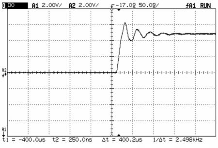
Figure 1: Ringing from mismatched impedances.

Clearly, if the signal overshoots or undershoots by enough then wrong data can get latched. The system crashes, people die and you've barricaded yourself behind the entrance as a reporter from 60 Minutes pounds on the doorbell.

It gets worse. Most of the logic we use today is CMOS, which offers decent performance for minimal power consumption. When the input to a CMOS gate goes somewhat more positive than the power supply (as that overshoot in Figure 1 does) the device goes into "SCR latchup." It tries to connect power to ground through its internal transistors. That works for a few milliseconds. Then the part self destructs from heat.

Don't believe me? Back when I was in the in-circuit emulator business we finally shipped the first of a new line of debuggers. This 64180 emulator ran at a paltry 6 MHz, but we drove signals to the user's target board very fast, with quite short rise times. The impedance of the customer's board was very different than our emulator; the overshoot drove his chips into SCR latchup. Every IC on his board quite literally exploded, plastic debris scattering like politicians dodging Michael Moore.

As I recall we never got paid for that emulator.

Firmware Implications

Work with your board developers to insure that the design not only works, but is debuggable. You'll hang all sorts of debug and test tools onto nodes on the board to get the code working properly. In-circuit emulators, for instance, connect to many dozens of very fast signals, and always create some sort of impedance mismatch.

Resistors are your friend. It's easy to add a couple of impedance-matching resistors, called terminators, at the receiving end of a driven line. Commonly used values are 220 ohms for the pullup resistor and 270 ohms for the one to ground. Since the power supply has a low impedance (otherwise the voltage to the chips would swing wildly as the load changes) the two resistors are essentially in parallel. With the values indicated the line sees about 120 ohms, not a bad value for most circuits.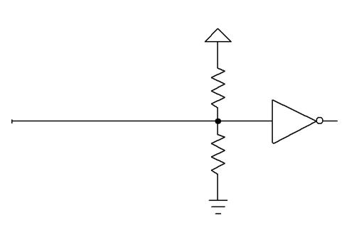

Figure 2 - Termination resistors at the end of a driven line match impedances.

These will greatly increase the power consumption of the board. An alternative is to replace the bottom resistor with a small, couple of hundred picofarad, capacitor.

Make sure the designers put terminations on critical signals. Any edge-triggered input to the processor (or to the circuit board) is particularly susceptible to electromagnetic-induced noise and reflections. For instance non-maskable interrupt is often edge-triggered. Without termination the slight impedance change resulting from connecting a tool to the line may cause erratic and mysterious crashes.

Many processors reduce pin counts using a multiplexed bus. The CPU supplies the address first, while asserting a strobe named ALE (address latch enable), AS (address strobe) or something similar. External logic latches the value into a register. Then the processor transfers data over the same pins. Just a bit of corruption of ALE will - once in a while - cause the register to latch the wrong information. Without termination, connecting a tool may give you many joyous days of chasing ghostly problems that appear only sporadically.

Clocks are an ever-increasing source of trouble. Most designs use a single clock source that drives perhaps dozens of chips. There's little doubt that the resulting long clock wire will be rife with reflections, destroying its shape. Unfortunately, most CPUs are quite sensitive to the shape and level of clock.

But it's generally not possible to use a termination network on clock, as many CPUs need a clock whose "one" isn't a standard logic level. It's far better to use a single clock source that drives a number of buffers, each of which distribute it to different parts of the board. To avoid skew (where the phase relationship of the signal is a bit different between each of the resulting buffer outputs), use a single buffer chip to produce these signals.

One of my favorite tools for debugging firmware problems is the oscilloscope. A mixed-signal scope, which combines both analog and digital channels, is even better. But scopes lie. Connect the instrument's ground via a long clip lead and the displayed signal will be utterly corrupt since Fourier frequencies far in excess of what you're measuring turn long ground wires into complex transmission lines.

Use that short little ground lead at the end of the probe! and things might not get much better. As speeds increase that 3 inch wire starts to look like an intricate circuit. Cut it shorter. Or remove the ground lead entirely and wrap a circle of wire around the probe's metal ground sheath. The other end gets soldered to the PCB, and is as short as is humanly possible.

A Reference

After staggering through those electromagnetics classes I quickly sold the textbooks. They were pretty nearly written in some language I didn't speak, one as obscure to me as Esperanto.

But there is a book that anyone with a bit of grounding in electronics can master, that requires math no more complex than algebra: High-Speed Digital Design: A Handbook of Black Magic, by Howard Johnson and Martin Graham, 1993, PTR Prentice Hall, Englewood Cliffs, NJ.

Reviewers on Amazon love the book or hate it. Me, I find it readable and immediately useful. The work is for the engineer who simply has to get a job done. It's not theoretical at all and presents equations without derivations. But it's practical.

And as for theoretical electromagnetics? My son goes to college to study physics in the Fall. I've agreed to write the checks if he answers my physics questions. Maybe in a few years he'll be able to finally explain Maxwell's Laws.

Till then you can pry my termination resistors from my cold, dead hands.