

Approximation Code for Roots, logs, and Exponentials, by Jack Ganssle
Do you need to compute roots or exponentials in your embedded systems firmware? This article gives the code needed to compute square and cube roots, logarithms, and exponentials (powers of 2, e, and 10).
I also wrote about computing approximations for trig functions here.
In the early embedded days Real Programmers wrote their code in assembly language. They knew exactly what the program did and how many clock cycles were required.
Then customers wanted systems that worked with real-world data. Floating point reared it's very ugly head. Anyone can do integer math in assembly, but floats are tough indeed.
Possibly the first solution was written by one C. E. Ohme. He contributed the source of a floating point library to Intel's Insite library, a free service that far predated the open source movement. This was long before the Internet so Intel sent hard-copy listings to developers. One could also order the source on media - punched paper tape!
Ohme's package did the four basic bits of arithmetic on 32 bit floats, astonishingly using only 768 bytes of ROM. That's remarkable considering the 8008's limited instruction set which had a hardware stack only seven levels deep.
Then customers wanted systems that did real-world computations. Roots and trig, logs and exponentiation were suddenly part of many embedded systems.
Today we hardly think about these constructs. Need to take the cosine of a number? Include math.h and use double cos(double). Nothing to it. But that's not so easy in assembly language unless the processor has built-in floating point instructions, a rare thing in the embedded space even now. So developers crafted a variety of packages that computed these more complex functions. To this day these sorts of routines are used in compiler runtime libraries. They're a great resource that gives us a needed level of abstraction from their grimy computational details.
But the packages unfortunately isolate us from these grimy computational details, which can lead to significant performance penalties. A fast desktop with built-in floating point hardware can return a cosine in a few tens of nanoseconds. But the same function often takes many milliseconds on embedded systems.
Or even longer. Everyone recognizes that to do a double-precision trig function (as required by the C standard) would take about a week on an 8051, so most of those compilers cheat and return shorter floats.
Compiler vendors are in the unenviable position of trying to provide a runtime library that satisfies most users. Yet in the embedded world we often have peculiar requirements that don't align with those of the rest of the world. What if you need a really speedy cosine. . . . but don't require a lot of precision? A look-up table is fast, but when accurate to more than a couple of decimal digits grows in size faster than Congressional pork.
Approximations in General
Most of the complicated math functions we use compute what is inherently not computable. There's no precise solution to most trig functions, square roots, and the like, so libraries employ approximations of various kinds. We, too, can employ various approximations to meet peculiar embedded system requirements.
College taught us that any differentiable function can be expressed by a Taylor series, such as:
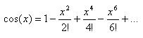
Like all approximations used in runtime packages, this is simply a polynomial that's clear, simple and easy to implement. Unhappily it takes dozens of terms to achieve even single precision float accuracy, which is an enormous amount of computation.
Plenty of other series expansions exist, many of which converge to an accurate answer much faster than the Taylor series. Entire books have been written on the subject and one could spend years mastering the subject.
But we're engineers, not mathematicians. We need cookbook solutions now. Happily computer scientists have come up with many.
The best reference on the subject is the suitably titled "Computer Approximations," by John Hart et al, Second Edition, 1978, Robert Krieger Publishing Company, Malabar, FL. It contains thousands of approximations for all of the normal functions like roots, exponentials, and trig, as well as approaches for esoteric relations like Bessel Functions and Elliptic Integrals. It's a must-have for those of us working on real-time resource-constrained systems.
But it's out of print. You can pry my copy out of my cold, dead fingers when my wetwear finally crashes for good. As I write this there are 6 copies from Amazon Marketplace for about $250 each. Long ago I should have invested in Google, Microsoft.. . . and Computer Approximations!
Be warned: it's written by eggheads for eggheads. The math behind the derivation of the polynomials goes over my head.
Tables of polynomial coefficients form the useful meat of the book. Before each class of function (trig, roots, etc) there's a handful of pages with suggestions about using the coefficients in a program. Somewhere, enigmatically buried in the text, like an ancient clue in a Dan Brown thriller, an important point about actually using the coefficients lies lost. So here's how to interpret the tables: An "index" vectors you to the right set of tables. An index for square roots looks like this:
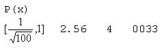
Which means: the set of coefficients labeled "0033" is for a polynomial of degree 4, accurate to 2.56 decimal digits for inputs between ![]() and 1. Outside that range all bets are off. The polynomial is of the form P(x). (Several other forms are used, like P(x)/Q(x), so that bit of what seems like pedantry is indeed important.)
and 1. Outside that range all bets are off. The polynomial is of the form P(x). (Several other forms are used, like P(x)/Q(x), so that bit of what seems like pedantry is indeed important.)
This is the corresponding table of coefficients:
  P00 (+ 0) +0.14743 837
  P01 (+ 1) +0.19400 802
  P02 (+ 1) -0.26795 117
  P03 (+ 1) +0.25423 691
  P04 (+ 0) -0.95312 89
The number in parenthesis is the power of ten to apply to each number. Entry P02, prefixed by (+1), is really -2.6795117.
It took me a long time to figure that out.
Knowing this the polynomial for the square root of x, over that limited range, accurate to 2.56 digits is:
![]()
It looks like a lot of trouble for a not-particularly accurate way to figure roots. The genius of this book, though, is that he lists so many variations (90 for square roots alone) that you can make tradeoffs to select the right polynomial for your application.
Three factors influence the decision: required accuracy, speed, and range. Like all good engineering predicaments, these conspire against each other. High speed generally means lower accuracy. Extreme accuracy requires a long polynomial that will burn plenty of CPU cycles, or a microscopic range. For instance, the following coefficients express 2x to 24.78 decimal digits of accuracy:
  P00 (+ 1) +0.72134 75314 61762 84602 46233 635
  P01 (- 1) +0.57762 26063 55921 17671 75
  Q00 (+ 2) +0.20813 69012 79476 15341 50743 885
  Q01 (+ 1)	+0.1
. . . . using the polynomial:
A bit of clever programming yields a routine that is surprisingly fast for such accuracy. Except that the range of x is limited to 0 to 1/256, which isn't particularly useful in most applications.
The trick is to do a bit of magic to the input argument to reduce what might be a huge range to one that satisfies the requirements of the polynomial. Since the range reduction process consumes CPU cycles it is another factor to consider when selecting an approximation.
Hart's book does describe range reduction math. in a manner an academic would love. But by puzzling over his verbiage and formulas, with some doodling on paper, it's not too hard to construct useful range reduction algorithms.
Roots
For example, I find the most useful square root polynomials require an input between 0.25 and 1. Since ![]() we can keep increasing k till
we can keep increasing k till ![]() is in the required range. Then use the polynomial to take the square root, and adjust the answer by 2k. Sidebar A implements the algorithm.
is in the required range. Then use the polynomial to take the square root, and adjust the answer by 2k. Sidebar A implements the algorithm.
Here's a sampling of interesting polynomials for square roots. Note that they can all be used with the range reduction scheme I've described.
With just two terms, using the form P(x) over the range [1/100, 1], this one is accurate to 0.56 decimal digits and is very fast:
  P00 (+0) +0.11544 2
  P01 (+1) +0.11544 2
A different form ![]() gives 3.66 digits over1/4 to 1:
gives 3.66 digits over1/4 to 1:
  P00 (- 1) +0.85805 2283
  P01 (+ 1) +0.10713 00909
  P02 (+ 0) +0.34321 97895
  Q00 (+ 0) +0.50000 08387
  Q01 (+ 1) +0.1
The following yields 8.95 digits accuracy using![]() , but works over the narrower 1/2 to 1 range. Use the usual range reduction algorithm to narrow x to 0.25 to 1, and then double the result if it's less than 1/2. Scale the result by the square root of two:
, but works over the narrower 1/2 to 1 range. Use the usual range reduction algorithm to narrow x to 0.25 to 1, and then double the result if it's less than 1/2. Scale the result by the square root of two:
    P00 (+ 0) +0.29730 27887 4025
  P01 (+ 1) +0.89403 07620 6457
  P02 (+ 2) +0.21125 22405 69754
  P03 (+ 1) +0.59304 94459 1466
  Q00 (+ 1) +0.24934 71825 3158
  Q01 (+ 2) +0.17764 13382 80541
  Q02 (+ 2) +0.15035 72331 29921
  Q03 (+ 1) +0.1
Hart's book also contains coefficients for cube roots. Reduce the argument's range to 0.5 to 1 (generally useful with his cube root approximations) using the relation: ![]() . See Sidebar B for details.
. See Sidebar B for details.
With just two terms in the form P(x) these coefficients give a cube root accurate to 1.24 digits over the range 1/8 to 1:
  P00 (+ 0) +0.45316 35
  P01 (+ 0) +0.60421 81
Adding a single term improves accuracy to 3.20 digits over 1/2 to 1:
  P00 (+ 0) +0.49329 5663
  P01 (+ 0) +0.69757 0456
  P02 (+ 0) -0.19150 216
Kick accuracy up by more than a notch, to 11.75 digits over 1/2 to 1 using the form :![]()
  P00 (+ 0) +0.22272 47174 61818
  P01 (+ 1) +0.82923 28023 86013 7
  P02 (+ 2) +0.35357 64193 29784 39
  P03 (+ 2) +0.29095 75176 33080 76
  P04 (+ 1) +0.37035 12298 99201 9
  Q00 (+ 1) +0.10392 63150 11930 2
  Q01 (+ 2) +0.16329 43963 24801 67
  Q02 (+ 2) +0.39687 61066 62995 25
  Q03 (+ 2) +0.18615 64528 78368 42
  Q04 (+ 1) +0.1
Sidebar A: Code to reduce the range of a Square Root
/***************************************************
*
*  reduce_sqrt - The square root routines require an input argument in
* the range[0.25, 1].This routine reduces the argument to that range.
*
* Return values:
* - "reduced_arg", which is the input arg/2^(2k)
* - "scale", which is the sqrt of the scaling factor, or 2^k
*
* Assumptions made:
* - The input argument is > zero
* - The input argument cannot exceed +2^31 or be under 2^-31.
*
* Possible improvements:
* - To compute a* 2^(-2k)) we do the division (a/(2^2k)). It's
*   much more efficient to decrement the characteristic of "a"
*  (i.e., monkey with the floating point representation of "a")
*   the appropriate number of times. But that's far less portable
*   than the less efficient approach shown here.
*
* How it works:
*  The algorithm depends on the following relation:
* sqrt(arg)=(2^k) * sqrt(arg * 2^(-2k))
*
*  We pick a "k" such that 2^(-2k) * arg is less than 1 and greater
*  than 0.25.
*
*  The ugly "for" loop shifts a one through two_to_2k while shifting a long
* version of the input argument right two times, repeating till the long
* version is all zeroes. Thus, two_to_2k and the input argument have
* this relationship:
*
*        two_to_2k        input argument         sqrt(two_to_2k)
*        4                1 to 4                 2
*        16               5 to 16                4
*        64               17 to 64               8
*        256              65 to 256             16
*
*  Note that when we're done, and then divide the input arg by two_to_2k,
* the result is in the desired [0.25, 1] range.
*
*  We also must return "scale", which is  sqrt(two_to_2k), but we prefer
* not to do the computationally expensive square root. Instead note
* (as shown in the table above) that scale simply doubles with each iteration.
*
*  There's a special case for the input argument being less than the [0.25,1]
* range. In this case we multiply by a huge number, one sure to bring
* virtually every argument up to 0.25, and then adjust
* "scale" by the square root of that huge number.
*
***************************************************/
void reduce_sqrt(double arg, double *reduced_arg, double *scale){
  long two_to_2k;              // divisor we're looking for: 2^(2k)
  long l_arg;                  // long (32 bit) version of input argument
  const double huge_num=1073741824;    // 2**30
  const double sqrt_huge_num= 32768;   // sqrt(2**30)
  if(arg>=0.25){
    // shift arg to zero while computing two_to_2k as described above
    l_arg=(long) arg;          // l_arg is long version of input arg
    for(two_to_2k=1, *scale=1.0; l_arg!=0; l_arg>>=2, two_to_2k<<=2,
     *scale*=2.0);
    // normalize input to [0.25, 1]
     *reduced_arg=arg/(double) two_to_2k;
    }else
     {
     // for small arguments:
     arg=arg*huge_num;           // make the number big
     l_arg=(long) arg;           // l_arg is long version of input arg
     for(two_to_2k=1, *scale=1.0; l_arg!=0; l_arg>>=2, two_to_2k<<=2,
      *scale*=2.0);
     *scale=*scale/sqrt_huge_num;
     // normalize input argument to [0.25, 1]
     *reduced_arg=arg/(double) two_to_2k;
     };
};
Sidebar B: Code to reduce the range of a cube root
/***************************************************
*
*  reduce_cbrt - The cube root routines require an input argument in
*  the range[0.5, 1].This routine reduces the argument to that range.
*
* Return values:
* - "reduced_arg", which is the input arg/2^(3k)
* - "scale", which is the cbrt of the scaling factor, or 2^k
*
* Assumptions made:
* - The input argument cannot exceed +/-2^31 or be under +/-2^-31.
*
* Possible improvements:
* - To compute a* 2^(-3k)) we do the division (a/(2^3k)). It's
*   much more efficient to decrement the characteristic of "a" (i.e.,
*   monkey with the floating point representation of "a") the
*   appropriate number of times. But that's far less portable than
*   the less efficient approach shown here.
* - Corections made for when the result is still under 1/2 scale by
*   two. It's more efficient to increment the characteristic.
*
* How it works:
*  The algorithm depends on the following relation:
*  cbrt(arg)=(2^k) * cbrt(arg * 2^(-3k))
*
*  We pick a "k" such that 2^(-3k) * arg is less than 1 and greater
* than 0.5.
*
*  The ugly "for" loop shifts a one through two_to_3k while shifting
* a long version of the input argument right three times, repeating
* till the long version is all zeroes. Thus, two_to_3k and the input
* argument have this relationship:
*
*        two_to_3k          input argument          cbrt(two_to_3k)
*        8                  1 to 7                  2
*        64                 8 to 63                 4
*        512                64 to 511               8
*        4096               512 to 4095            16
*
*  Note that when we're done, and then divide the input arg by
* two_to_3k, the result is between [1/8,1]. The following algorithm
* reduces it to [1/2, 1]:
*
*  if (reduced_arg is between [1/4, 1/2])
*   -multiply it by two and correct the scale by the cube root of two.
*  if (reduced_arg is between [1/4, 1/2])
*   -multiply it by two and correct the scale by the cube root of two.
*
*  Note that the if the argument was between [1/8, 1/4] both of those
* "if"s will execute.
*
*  We also must return "scale", which is  cbrt(two_to_3k), but we
* prefer not to do the computationally expensive cube root. Instead
* note (as shown in the table above) that scale simply doubles with
* each iteration.
*
*  There's a special case for the input argument being less than the
* [0.5,1] range. In this case we multiply by a huge number, one
* sure to bring virtually every argument up to 0.5, and then adjust
* "scale" by the cube root of that huge number.
*
*  The code takes care of the special case that the cube root of a
* negative number is negative by passing the absolute value of the
* number to the approximating polynomial, and then making "scale"
* negative.
*
***************************************************/
void reduce_cbrt(double arg, double *reduced_arg, double *scale){
   long two_to_3k;              // divisor we're looking for: 2^(3k)
   long l_arg;                  // 32 bit version of input argument
   const double huge_num=1073741824;      // 2**30
   const double cbrt_huge_num= 1024;      // cbrt(2**30)
   const double cbrt_2= 1.25992104989487; // cbrt(2)
   *scale=1.0;
   if(arg<0){                   // if negative arg, abs(arg) and set
     arg=fabs(arg);             //  scale to -1 so the polynomial
     *scale=-1.0;               //  routine will give a neg result
     };

   if(arg>=0.5){
     // shift arg to zero while computing two_to_3k as described above
     l_arg=(long) arg;          // l_arg is long version of input arg
     for(two_to_3k=1; l_arg!=0; l_arg>>=3, two_to_3k<<=3, *scale*=2.0);
     *reduced_arg=arg/(double) two_to_3k; // normalize to [0.5, 1]
     if(*reduced_arg<0.5){      // if in [1/8,1/2] correct it
       *reduced_arg*=2;
       *scale/=cbrt_2;
   };
   if(*reduced_arg<0.5){      // if in the range [1/4,1/2] correct it
     *reduced_arg*=2;
     *scale/=cbrt_2;
   };
 }else
   {
   // for small arguments:
   arg=arg*huge_num;          // make the number big
   l_arg=(long) arg;          // l_arg is long version of input arg
   for(two_to_3k=1; l_arg!=0; l_arg>>=3, two_to_3k<<=3, *scale*=2.0);
     *scale=*scale/cbrt_huge_num;


     if(*reduced_arg<0.5){         // if in [1/8,1/2] correct it
       *reduced_arg*=2;
       *scale/=cbrt_2;
     };
     if(*reduced_arg<0.5){         // if in [1/4,1/2] correct it
       *reduced_arg*=2;
       *scale/=cbrt_2;
     };
  };
};
Exponentiations
The three most common exponentiations we use are powers of two, e and 10. In a binary computer it's trivial to raise an integer to a power of two, but floating point is much harder. Approximations to the rescue!
Hart's power-of-two exponentials expect an argument in the range [0.0, 0.5]. That's not terribly useful for most real-world applications so we must use a bit of code to reduce the input "x" to that range.
Consider the equation ![]() . Well, duh. That appears both contrived and trite. Yet it's the basis for our range reduction code. The trick is to select an integer "a" so that "x" is between 0 and 1. An integer, because it's both trivial and fast to raise two to any int. Simply set "a" to the integer part of "x," and feed (x-int(x)) in to the approximating polynomial. Multiply the result by the easily computed 2a to correct for the range reduction.
. Well, duh. That appears both contrived and trite. Yet it's the basis for our range reduction code. The trick is to select an integer "a" so that "x" is between 0 and 1. An integer, because it's both trivial and fast to raise two to any int. Simply set "a" to the integer part of "x," and feed (x-int(x)) in to the approximating polynomial. Multiply the result by the easily computed 2a to correct for the range reduction.
But I mentioned that Hart wants inputs in the range [0.0, 0.5], not [0.0, 1.0]. If (x-int(a)) is greater than 0.5 use the relation:
![]()
instead of the one given earlier. The code is simpler than the equation. Subtract 0.5 from "x" and then compute the polynomial for (x-int(x)) as usual. Correct the answer by ![]() .
.
Exponents can be negative as well as positive. Remember that![]() . Solve for the absolute value of "x" and then take the reciprocal.
. Solve for the absolute value of "x" and then take the reciprocal.
Though I mentioned it's easy to figure 2a, that glib statement slides over a bit of complexity. The code listed in Sidebar A uses the worst possible strategy: it laboriously does floating point multiplies. That's a very general solution that's devoid of confusing chicanery so is clear, though slow.
Other options exist. If the input "x" never gets very big, use a look-up table of pre-computed values. Even a few tens of entries will let the resulting 2x assume huge values.
Another approach simply adds "a" to the number's mantissa. Floating point numbers are represented in memory using two parts, one fractional (the characteristic), plus an implied two raised to the other part, the mantissa. Apply "a" to the mantissa to create 2a. That's highly non-portable but very fast.
Or, one could shift a "one" left through an int or long "a" times, and then convert that to a float or double.
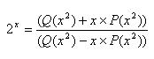
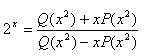
Computer Approximations lists polynomials for 46 variants of 2x, with precisions ranging from four to 25 decimal digits. Room (and sanity) prohibits listing them all. But here are two of the most useful examples. Both assume the input argument is between 0 and 0.5, and both use the following ratio of two polynomials:
The following coefficients yield a precision of 6.36 decimal digits. Note that P(x) is simply an offset, and Q01 is 1, making this a very fast and reasonably accurate approximation:
 P00 (+ 1) +0.86778 38827 9
 Q00 (+ 2) +0.25039 10665 03
 Q01 (+ 1) +0.1
For 10.03 digits of precision use the somewhat slower:
 P00 (+ 1) +0.72151 89152 1493
 P01 (- 1) +0.57690 07237 31
 Q00 (+ 2) +0.20818 92379 30062
 Q01 (+ 1) +0.1
If you're feeling a need for serious accuracy try the following coefficients, which are good to an astonishing 24.78 digits. But need a more complex range reduction algorithm to keep the input between [0, 1/256]:
 P00 (+ 1) +0.72134 75314 61762 84602 46233 635
 P01 (- 1) +0.57762 26063 55921 17671 75
 Q00 (+ 2) +0.20813 69012 79476 15341 50743 885
 Q01 (+ 1)	+0.1
Note that the polynomials, both of degree 1 only, quickly plop out an answer.
Other Exponentials
What about the more common natural and decimal exponentiations? Hart lists many, accurate over a variety of ranges. The most useful seem to be those that work between [0.0, 0.5] and [0.0, 1.0]. Use a range reduction approach much like that described above, substituting the appropriate base: 10x = 10a x 10(x-a)or ex = ea x e(x-a).
Using the same ratio of polynomials listed above the following coefficients give to 12.33 digits:
 P00 (+ 2) +0.41437 43559 42044 8307
 P01 (+ 1) +0.60946 20870 43507 08
 P02 (- 1) +0.76330 97638 32166
 Q00 (+ 2) +0.35992 09924 57256 1042
 Q01 (+ 2) +0.21195 92399 59794 679
 Q02 (+ 1) +0.1
The downside of using this or similar polynomials is you've got to solve for that pesky 10a. Though a look-up table is one fast possibility if the input stays in a reasonable range, there aren't many other attractive options. If you're working with an antique IBM 1602 BCD machine perhaps it's possible to left shift by factors of ten in a way analogous to that outlined above for exponents of 2. In today's binary world there are no left-shift decimal instructions so one must multiply by 10.
Instead, combine one of the following relations

with the power-of-two approximations listed above as shown in Sidebar C.
Logs
There's little magic to logs, other than a different range reduction algorithm. Again, it's easiest to develop code that works with logarithms of base 2. Note that:
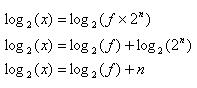
We pick an n that keeps f between [0.5, 1.0], since Hart's most useful approximations require that range. The reduction algorithm is very similar to that described last issue for square roots, and is shown in Sidebar D. Sidebar E gives code to compute log base 2 to 4.14 digits of precision.
Need better results? The following coefficients are good to 8.32 digits over the same range:
 P00 (+1) -.20546 66719 51
 P01 (+1) -.88626 59939 1
 P02 (+1) +.61058 51990 15
 P03 (+1) +.48114 74609 89
 Q00 (+0) +.35355 34252 77
 Q01 (+1) +.45451 70876 29
 Q02 (+1) +.64278 42090 29
 Q03 (+1) +.1
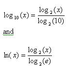
Though Hart's book includes plenty of approximations for common and natural logs, it's probably more efficient to compute and use the change of base formulas:
So far I've talked about the approximations' precision imprecisely. What exactly does precision mean? Hart chooses to list relative precision for roots and exponentials:
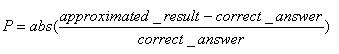
Logarithms are a different game altogether; he uses absolute precision, defined by:
P = abs(approximated_result-correct_answer)
To figure decimal digits of precision use:
Digits = 2 - log10 (P)
Computer Approximations includes polynomials for all of the standard and inverse trig functions and much more. See https://www.ganssle.com/approx/sincos.cpp for implementations of trig functions.
Converting Hart's terse range reduction explanations to useful algorithms does take a bit of work, but the book is an invaluable treasure for people faced with creating approximations. The samples I've shown just touch a fraction of a percent of the approximations contained in the book.
It's pretty cool to crank parameters into these simple equations that use such bizarre-looking coefficients, and to see astonishingly correct answers pop out every time.
(Please use proper engineering analysis when implementing these suggestions - no guarantees are given. This demo code is merely meant to illustrate algorithms.).
Sidebar A: Code to reduce the range of an exponential
/***************************************************
*
*  reduce_expb - The expb routines require an input argument in
* the range[0.0, 0.5].This routine reduces the argument to that range.
*
* Return values:
* - "arg", which is the input argument reduced to that range
* - "two_int_a", which is 2**(int(arg))
* - "adjustment", which is an integer flag set to zero if the
*   fractional part of arg is <=0.5; set to one otherwise
*
* How this range reduction code works:
*  (1) 2**x = 2**a * 2**(x - a)
* and,
*  (2) 2**x = 2**(1/2) * 2**a * 2**(x - a - 1/2)
*
*  Now, this all looks pretty contrived. But the trick is to pick an
* integer "a" such that the term (x - a) is in the range [0.0, 1.0].
* If the result is in the range we use equation 1. If it winds up in
* [0.5, 1.0], use equation (2) which will get it down to our desired
* [0.0, 0.5] range.
*
*  The return value "adjustment" tells the calling function if we
* are using the first or the second equation.
*
***************************************************/
void reduce_expb(double *arg, double *two_int_a, int *adjustment){
int int_arg; // integer part of the input argument
 *adjustment = 0;             // Assume we're using equation (2)
 int_arg =  (int) *arg;
 if((*arg - int_arg) > 0.5)   // if frac(arg) is in [0.5, 1.0]...
   {
       *adjustment = 1;
       *arg = *arg - 0.5;     // ... then change it to [0.0, 0.5]
   }
 *arg = *arg - (double) int_arg;   // arg == just the fractional part
// Now compute 2** (int) arg.
   *two_int_a = 1.0;
   for(; int_arg!=0; int_arg--)*two_int_a = *two_int_a * 2.0;
};
Sidebar B: 2x to 9.85 digits
/**************************************************
*
* expb1063 - compute 2**x to 9.85 digits accuracy
*
***************************************************/
double expb1063(double arg){
  const double P00 = + 7.2152891521493;
  const double P01 = + 0.0576900723731;
  const double Q00 = +20.8189237930062;
  const double Q01 = + 1.0;
  const double sqrt2= 1.4142135623730950488; // sqrt(2) for scaling
  double two_int_a;                  // 2**(int(a))
  int    adjustment;                 // set to 1 by reduce_expb
  // ...adjust the answer by sqrt(2)
  double answer;                     // The result
  double Q;                          // Q(x**2)
  double x_P;                        // x*P(x**2)
  int    negative=0;                 // 0 if arg is +; 1 if negative
//  Return an error if the input is too large. "Too large" is
// entirely a function of the range of your floating point
// library and expected inputs used in your application.
  if(abs(arg>100.0)){
     printf("\nYikes! %d is a big number, fella. Aborting.", arg);
     return 0;
  }
//  If the input is negative, invert it. At the end we'll take
// the reciprocal, since n**(-1) = 1/(n**x).
  if(arg<0.0)
  {
     arg = -arg;
     negative = 1;
  }
  reduce_expb(&arg, &two_int_a, &adjustment);// reduce to [0.0, 0.5]
// The format of the polynomial is:
//  answer=(Q(x**2) + x*P(x**2))/(Q(x**2) - x*P(x**2))
//
//  The following computes the polynomial in several steps:
  Q   =        Q00 + Q01 * (arg * arg);
  x_P = arg * (P00 + P01 * (arg * arg));
  answer= (Q + x_P)/(Q - x_P);

// Now correct for the scaling factor of 2**(int(a))
  answer= answer * two_int_a;

// If the result had a fractional part > 0.5, correct for that
  if(adjustment == 1)answer=answer * sqrt2;

// Correct for a negative input
  if(negative == 1) answer = 1.0/answer;
  return(answer);
};
Sidebar C: Computing 10x using a 2x approximation
/**************************************************
*
* expd_based_on_expb1063 - compute 10**x to 9.85 digits accuracy
*
*  This is one approach to computing 10**x. Note that:
* 10**x = 2** (x / log_base_10(2)), so
* 10**x = expb(x/log_base_10(2))
*
***************************************************/
double expd_based_on_expb1063(double arg){
   const double log10_2 = 0.30102999566398119521;
   return(expb1063(arg/log10_2));
}
Sidebar D - Log Range Reduction Code
/***************************************************
*
*  reduce_log2 - The log2 routines require an input argument in
* the range[0.5, 1.0].This routine reduces the argument to that range.
*
* Return values:
* - "arg", which is the input argument reduced to that range
* - "n", which is n from the discussion below
* - "adjustment", set to 1 if the input was < 0.5
*
* How this range reduction code works:
*  If we pick an integer n such that x=f x 2**n, and 0.5<= f < 1, and
* assume all "log" functions in this discussion means log(base 2),
* then:
* log(x) = log(f x 2**n)
*        = log(f) + log(2**n)
*        = log(f) + n
*
*  The ugly "for" loop shifts a one through two_to_n while shifting a
* long version of the input argument right, repeating till the long
* version is all zeroes. Thus, two_to_n and the input argument have
* this relationship:
*
*       two_to_n        input argument           n
*        1                0.5 to 1               0
*        2                  1 to 2               1
*        4                  2 to 4               2
*        8                  4 to 8               3
* etc.
*
*  There's a special case for the argument being less than 0.5.
* In this case we use the relation:
*  log(1/x)=log(1)-log(x)
*          =      -log(x)
* That is, we take the reciprocal of x (which will be bigger than
* 0.5) and solve for the above. To tell the caller to do this, set
* "adjustment" = 1.
*
***************************************************/
void reduce_log2(double *arg, double *n, int *adjustment){
  long two_to_n;               // divisor we're looking for: 2^(2k)
  long l_arg;                  // long (32 bit) version of input
  *adjustment=0;
  if(*arg<0.5){                // if small arg use the reciprocal
     *arg=1.0/(*arg);
     *adjustment=1;
  }
  // shift arg to zero while computing two_to_n as described above
  l_arg=(long) *arg;            // l_arg = long version of input
  for(two_to_n=1, *n=0.0; l_arg!=0; l_arg>>=1, two_to_n<<=1, *n+=1.0);
  *arg=*arg / (double) two_to_n;// normalize argument to [0.5, 1]
};
Sidebar E: Log base 2 code good to 4.14 digits
/**************************************************
*
* LOG2_2521 - compute log(base 2)(x) to 4.14 digits accuracy
*
***************************************************/
  double log2_2521(double arg){
  const double P00 = -1.45326486;
  const double P01 = +0.951366714;
  const double P02 = +0.501994886;
  const double Q00 = +0.352143751;
  const double Q01 = +1.0;
  double n;                            // used to scale result
  double poly;                         // result from polynomial
  double answer;                       // The result
  int    adjustment;                   // 1 if argument was < 0.5

//  Return an error if the input is <=0 since log is not real at and
// below 0.
  if(arg<=0.0){
     printf("\nHoly smokes! %d is too durn small. Aborting.", arg);
     return 0;
  }
  reduce_log2(&arg, &n, &adjustment);   // reduce  to [0.5, 1.0]
// The format of the polynomial is P(x)/Q(x)
  poly= (P00 + arg * (P01 + arg * P02)) / (Q00 + Q01 * arg);

// Now correct for the scaling factors
  if(adjustment)answer = -n - poly;
  else answer=poly + n;
  return(answer);
};